Georeferencing Ordnance Survey Maps

The British Library has digitised over 10,500 historical Ordnance Survey (OS) maps as part of the Living with Machines project (to know more about the selection process you can read our blogpost on Digitising Ordnance Survey maps). 

These maps were digitised as TIFF files – a high-quality format that is standard in libraries and archives. However, in order to make them usable for research purposes, we had to create GeoTIFF files. 

GeoTIFFs are files that include geospatial metadata (geographical coordinates), e.g. information that makes it possible to position a map on the earth’s surface. 

This blogpost outlines how Giorgia Tolfo georeferenced this important new contribution to the digitised OS collection. 

How do we transform TIFFs into GeoTIFFs?

This transformation is often called georeferencing. To georeference a map, one identifies ‘control points’, or locations on a map that can confidently be assigned latitude and longitude coordinates. There are many approaches to georeferencing. Choices about how a map is georeferenced can impact its future usability. In this case, georeferencing is difficult largely because of the number of maps: locating control points is a time-intensive task. Our approach to georeferencing these OS sheets was therefore based on using the four corners of the map as control points. 

This resulted in a rectangle whose corner points have been geolocated, as shown by the figure below.

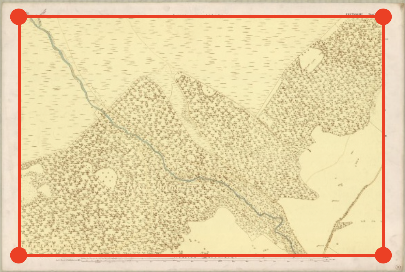
Fig 1. OS Maps 25″ 1st edition. Perth and Clackmannanshire XXI.10 (Blair Athole). Survey date: 1861, Publication date: 1867.

Where do we get the coordinates?

Using the corners as control points was a timesaver because of the simplicity of selecting these on the image. But owing to pre-existing data, ultimately, the biggest advantage to this method was that we already knew the geocoordinates for these corners – we didn’t have to look them up ourselves!

This was possible because NLS shared a file of metadata that includes predicted corner locations for every sheet printed by the OS. This information was obtained from Ed Fielden and his Coordinate Converter website, where the relevant OS County Series projection and coordinate information is made available.

Here is an example of a record with such geocoordinates.

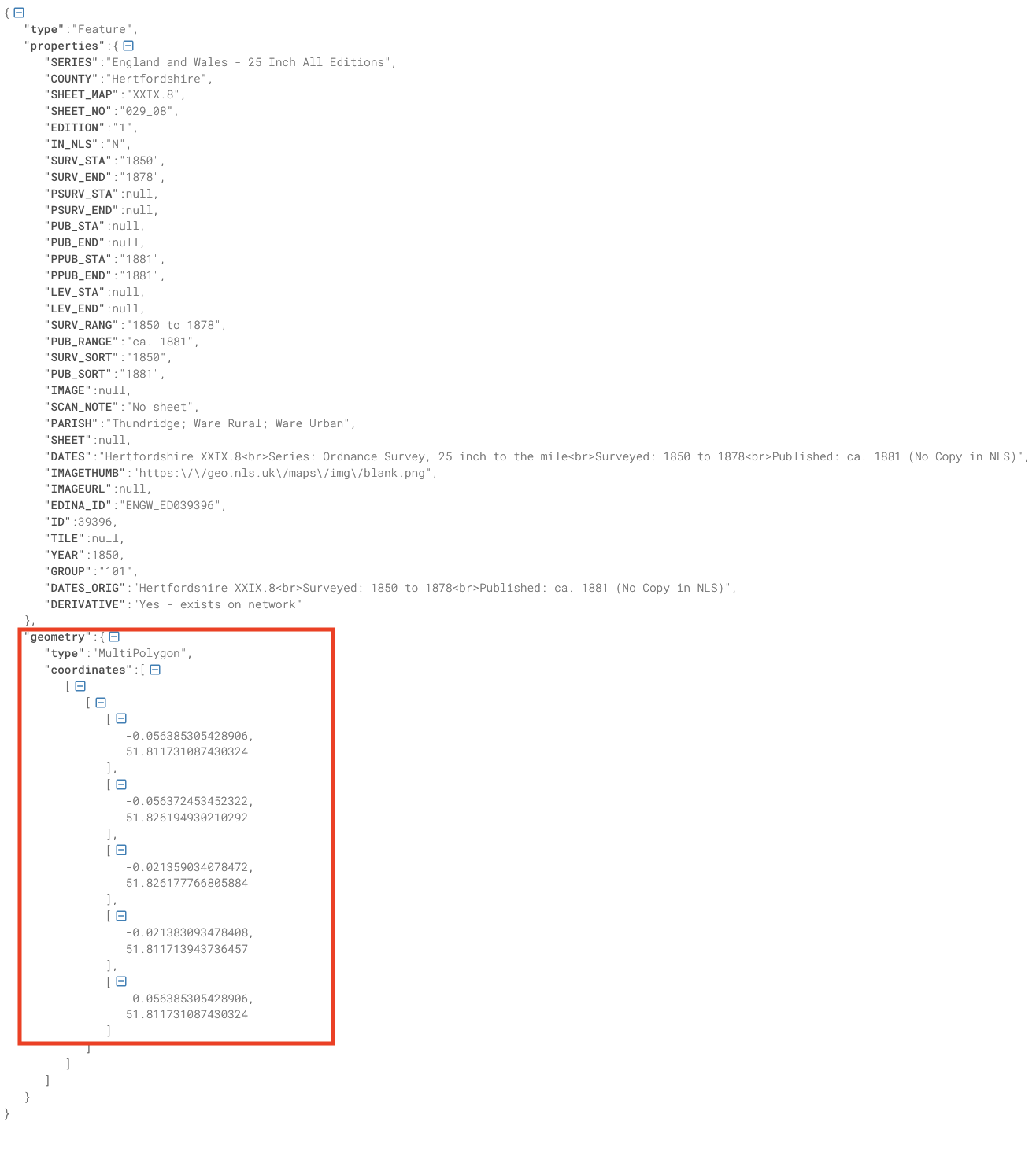
Fig 2. Example of JSON file including sheet metadata shared by the NLS.

How do we connect everything?

So, we have maps (TIFFs) and we have metadata (JSON files). Now we need to combine them, to create GeoTIFFs to create GeoTIFFs.

The solution we adopted was designed by the British Library’s British Library’s Digital Mapping Lead Curator, Gethin Rees. 

The code, developed while working on 1-inch Old Series Ordnance Survey maps of England and Wales and 1-inch Survey of India maps, worked on the assumption that the image filename included basic metadata for linking image files to metadata files. With sheet and subsheet number it is in fact possible to associate the image file to the correct metadata entry.

Taking this code as a starting point, Tolfo, with the help of the BL Labs Technical Lead Filipe Bento, updated it to be able to use it with different OS maps.

Now we can run the code! This creates a visual interface where it’s possible to select points on the image of the scanned map. By clicking on the four corners of a map, we can associate the geocoordinates with these image coordinates. (The selected corners are not of the edges of the paper sheet, but of the ‘mapped’ content, e.g. the map inside the neatline.)

Is that it?

Unfortunately not… 

To georeference the images, we needed a human to click on the corners of the map images. So Tolfo went through all the maps to select their corners. 

Fantastic. Is that it?

Unfortunately, again, this is not the end. 

While it’s easy to think about the maps as individual sheets that can all be stitched together into a national map (as the NLS has beautifully done with some of their OS collections), in fact there are several reasons this step is very, very difficult. 

OS map collections include some peculiar additions: 

1. Masked content
2. Insets
3. Index sheets

Historically, masked content and index sheets exist because sometimes the maps were printed in volumes destined for specific audiences. In the case of the maps held at the British Library, these were bound in volumes as part of the ‘County Series’. County Series maps focused on showing maps for just one county at a time (Lancashire, Kent, etc.). On these maps, details for areas of the map beyond the county boundary were masked, or removed, like in the example below, where Northumberland is blank.

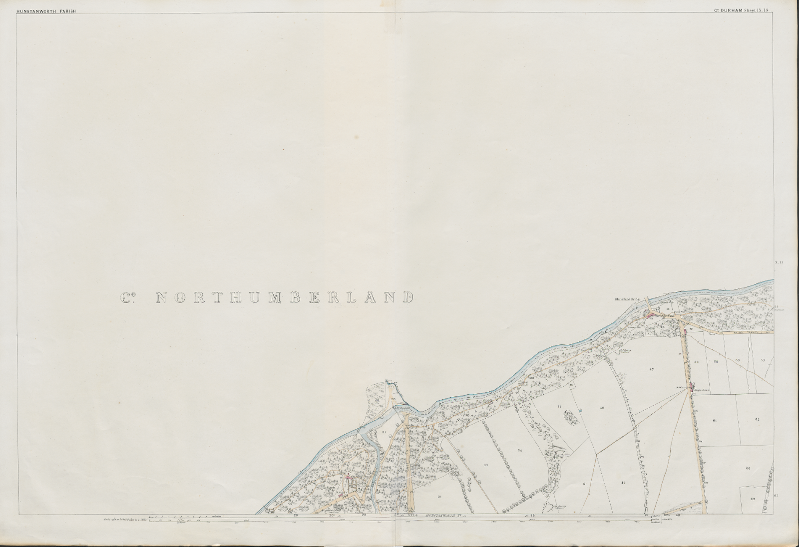
Fig 3. OS Maps 25″ 1st edition. Durham IX.16 Surveyed: ca. 1855 to 1856. Published: ca. 1875. 

In addition, maps can have insets. Insets like the one shown below prevented needing another sheet just to show a tiny piece of land. These are especially common for coastal areas.

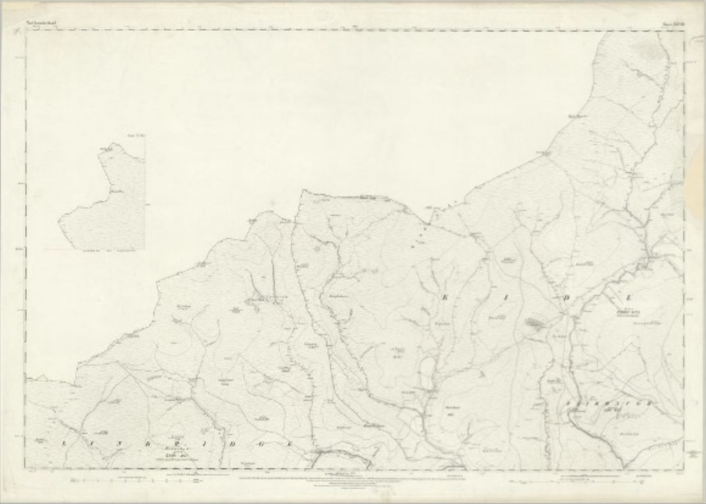
Fig 4. OS Maps 25″ 1st edition. Northumberland Sheet XXVIII (inset XXVIIIA) Surveyed: 1861 to 1863, Published: 1866.

Finally, index sheets represent the coverage of the maps bound within the volumes for counties: they were used like a table of contents for each county set, helping map users find the map of interest for their query.

These exceptions are not easy to georeference. In the best cases, they can produce duplicates, while in more difficult ones they would require creating cutouts from sheets to distinguish between land that sits within the coordinates of the four corners of the map and land that does not. If you’d like to learn more about the opportunities and challenges of working with digitised map collections, check out our article in the Journal of Victorian Culture as well as the MapReader software library (and paper).

What next….?

So far, we have georeferenced all the ‘standard’ maps, leaving duplicates, maps with insets, and indexes aside. 

Researchers interested in using the maps can contact British Library Labs.